Reconstructing scenes through fog, seeing through tissues in the human body, detecting cracks and material properties through paint and imaging through the atmosphere all require imaging through a medium that scatters light. We developed a set of fast, robust methods for the various stages of this imaging pipeline. Central to our work the problem of phase retrieval problem. Our methods have been used with next-generation photonic computing systems for fast machine learning with light.
Imaging process and challenges
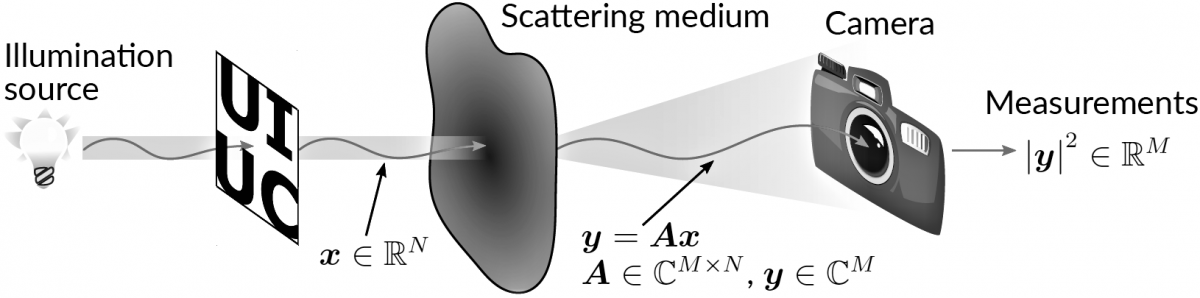
The object we are intersted in is illuminated and the light is scattered by a scattering medium (such as human body tissue). The resulting output complex-valued optical field, \( \boldsymbol{y} \in \mathbb{C}^M \), is related linearly to the (vectorized) object, \(\boldsymbol{x} \in \mathbb{R}^N\), by a typically unknown complex-valued transmission matrix, \(\boldsymbol{A} \in \mathbb{C}^{M \times N}\). We capture and measure the scattered light using a camera. Unfortunately typical camera sensors can only measure the elementwise intensity (magnitude), \(|\boldsymbol{y}|^2 \in \mathbb{R}^M\), and the phase of the complex-valued entries of \( \boldsymbol{y}\) is lost.
We aim to recover the input field, \( \boldsymbol{x}\), from intensity measurements, \( |\boldsymbol{y}|^2 \),
when the transmission matrix, \( \boldsymbol{A} \), is unknown.
Three steps
We design new methods and algorithms to do this in three stages:
- Measurement phase retrieval: Using known \( \boldsymbol{\Xi} \in \mathbb{R}^{N \times K}\), recover \( \boldsymbol{Y} \) from optical measurements \( |\boldsymbol{Y}|^2 = |\boldsymbol{A \Xi}|^2 \) with unknown \( \boldsymbol{A} \).
- Calibrate \( \boldsymbol{A} \): With \( \boldsymbol{Y} \) now known and \( \boldsymbol{\Xi} \) known from before, recover \( \boldsymbol{A}\) from a linear (not quadratic anymore!) system \(\boldsymbol{Y} = \boldsymbol{A \Xi} \).
- Recover \( \boldsymbol{x}\): Account for any errors in optical measurements, \( |\boldsymbol{y}|^2 \), and calibrated \( \boldsymbol{A} \) to recover \(\boldsymbol{x}\).
Our work is amongst the first to show measurement phase retrieval and account for errrors in calibrated \( \boldsymbol{A} \) for signal recovery. Transforming calibration of \( \boldsymbol{A} \) from a quadratic to a linear problem that is simple to solve is also novel. We verify all three steps in simulations and on real hardware that is used in optical computing.
Step 1: Measurement phase retrieval
Realizing that we can measure distances between points on the complex plane is the key to measurement phase retrieval. \(\def\abs#1{{|#1|}} \def\inprod#1{\left\langle#1\right\rangle} \def\R{\mathbb{R}} \def\C{\mathbb{C}} \def\vec#1{\boldsymbol{{#1}}} \def\mat#1{\boldsymbol{{#1}}} \def\va{\vec{a}} \def\vxi{\vec{\xi}} \def\vu{\vec{u}} \def\vv{\vec{v}} \def\mA{\mat{A}} \def\mY{\mat{Y}} \def\mXi{\mat{\Xi}} \def\mE{\mat{E}} \def\mM{\mat{M}} \def\mW{\mat{W}} \def\sfr{\mathsf{r}} \def\sfy{\mathsf{y}}\) To see this:
- Let \(\va \in \C^N\) be a row of \(\mA\).
- Let \(\vu\) and \(\vv\) be two (real or complex) signals.
- Denote the two complex-valued inner products \(y_1 = \inprod{\va, \vu} \) and \(y_2 = \inprod{\va, \vv} \)
- Now we interfere the two signals, \(\vu -\vv\).
- We then obtain the optical intensity measurement of the interfered signal, \(\abs{\inprod{\va, \vu-\vv}^2} = \abs{y_1 - y_2}^2\). This is the distance between two points on the complex plane!
With this in mind, we can interfere multiple signals with each other to optically measure pairwise distances between complex numbers. From these distances we can use Eucldiean distance geometry techiniques and locate a realization of points on the complex plane that satisfy these distances. The localized points are the complex-valued measurements (inner products) and their phase on the complex plane is the measurement phase.
Applications in optical computing
We can use measurement phase retrieval to do rapid machine learning and signal processing computations such as randomized linear algebra and dimensionality reduction on an optical processing unit:
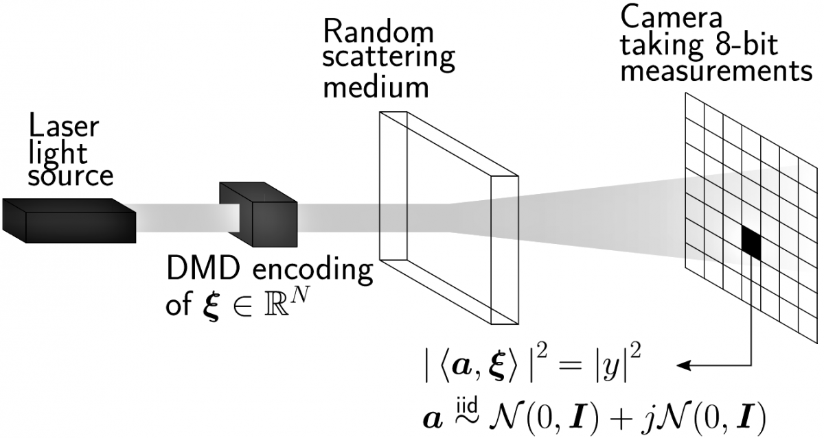
The optical processing unit does matrix-vector multiplication. It 'imprints' a signal, \(\vxi\), onto a coherent light beam using a digital micro-mirror device (DMD) which is then shined through a multiple scattering medium such as a white polymer layer. The elements of the transmission matrix of the scattering medium are unknown. However, the scattering medium acts like an iid standard complex Gaussian matrix. A camera with 8-bit precision measures the intensity of the scattered light.
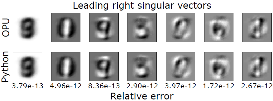
We use this hardware to perform randomized SVD. One step of the randomized SVD procedure requires multiplying the matrix whose SVD we want, \(\mXi\), with a random matrix, \(\mA\) and using the result. We perform this step using the optical processing unit to first obtain \(\abs{\mY}^2 = \abs{\mA \mXi}^2\). Then measurement phase retrieval is used to obtain the random matrix multplication result, \(\mY\). In our experminent \(\mXi\) is created by vectorizing and horizontally stacking MNIST images. The difference between using Python's built-in SVD routine and randomized SVD with measurment phase retreival is negligible. The below figure visualizes the right singular vectors:
Relevant publications
- Fast Optical System Identification by Numerical Interferometry
- Don't take it lightly: Phasing optical random projections with unknown operators
Step 2: Rapid transmission matrix calibration
After measurement phase retrieval, transmission matrix calibration is a simple linear problem instead of a quadratic problem. With \( \boldsymbol{Y} \) now known and \( \boldsymbol{\Xi} \) known from before, we recover \( \boldsymbol{A}\) from \(\boldsymbol{Y} = \boldsymbol{A \Xi} \) instead of \(\abs{\mY}^2 = \abs{\mA \mXi}^2 \). \(\def\abs#1{{|#1|}} \def\inprod#1{\left\langle#1\right\rangle} \def\R{\mathbb{R}} \def\C{\mathbb{C}} \def\vec#1{\boldsymbol{{#1}}} \def\mat#1{\boldsymbol{{#1}}} \def\va{\vec{a}} \def\vxi{\vec{\xi}} \def\vv{\vec{v}} \def\vx{\vec{x}} \def\vy{\vec{y}} \def\mA{\mat{A}} \def\mY{\mat{Y}} \def\mXi{\mat{\Xi}} \def\mE{\mat{E}} \def\mM{\mat{M}} \def\mW{\mat{W}} \def\sfr{\mathsf{r}} \def\sfy{\mathsf{y}} \DeclareMathOperator*{\argmin}{arg\,min}\)
One of the fastest method to calibrate \(\mA \in \C^{M \times N}\) from quadratic problem \(\abs{\mY}^2 = \abs{\mA \mXi}^2 \) takes \(3.26\) hours when \(N = 64^2\) and \(\frac{M}{N} = 16\). The following table reports the time taken to do measurement phase retrieval and recover \( \boldsymbol{A}\) from \(\boldsymbol{Y} = \boldsymbol{A \Xi} \) on the optical processing hardware. Our linear method is significantly faster.
| \(\boldsymbol{N}\) | \(\boldsymbol{M / N}\) | Time (minutes) |
|---|---|---|
| \(32^2\) | \(32\) | \(0.97\) |
| \(32^2\) | \(64\) | \(2.05\) |
| \(32^2\) | \(128\) | \(4.01\) |
| \(64^2\) | \(16\) | \(6.15\) |
| \(64^2\) | \(32\) | \(11.69\) |
| \(64^2\) | \(64\) | \(24.14\) |
| \(96^2\) | \(16\) | \(31.36\) |
| \(128^2\) | \(12\) | \(71.07\) |
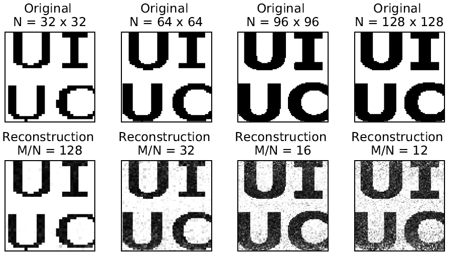
To verify that we have calibrated accurate transmission matrices, we use them for imaging through scattering media. A new signal, \(\vx \in \R^N\) which we assume is unknown, is inputted into the optical system to produce optical measurements \(\abs{\vy}^2 \in \R^M \). Using the calibrated \(\mA \in \C^{M \times N} \), we use the Wirtinger flow phase retrieval algorithm to obtain an estimate of \(\vx\) from \(\abs{\vy}^2 \). The following figure shows that we calibrate transmission matrices which can be used for imaging through scattering media. The image dimension, \(N\), and oversampling ratio, \(\frac{M}{N}\), is varied:
Applications in optical computing
Optical deep neural networks can replace traditional fully-connected neural network layers with an optical processing unit that can perform fast matrix-vector multiplications. This is particularly advantageous in modern machine learning applications where the dimension of our input data is growing. However, in order to train such neural networks and use backpropagation, the entries of the scattering medium in the optical processing unit are required. Our method enables these entries to be obtained rapidly.
Relevant publications
Further resources
Below is a lecture talk which explains measurement phase retrieval and rapid linear transmission matrix calibration. The slides from the talk are also available.
Step 3: Phase retrieval with operator error
After obtaining the transmission matrix, we wish to use it to recover new input signals from their quadratic measurements. \(\def\abs#1{{|#1|}} \def\inprod#1{\left\langle#1\right\rangle} \def\R{\mathbb{R}} \def\C{\mathbb{C}} \def\vec#1{\boldsymbol{{#1}}} \def\mat#1{\boldsymbol{{#1}}} \def\va{\vec{a}} \def\vxi{\vec{\xi}} \def\vu{\vec{u}} \def\vv{\vec{v}} \def\mA{\mat{A}} \def\mY{\mat{Y}} \def\mXi{\mat{\Xi}} \def\mE{\mat{E}} \def\mM{\mat{M}} \def\mW{\mat{W}} \def\sfr{\mathsf{r}} \def\sfy{\mathsf{y}}\) We aim to recover \( \vx \) from $$ \abs{\vy}^2 \approx \abs{\mA \vx}^2. $$
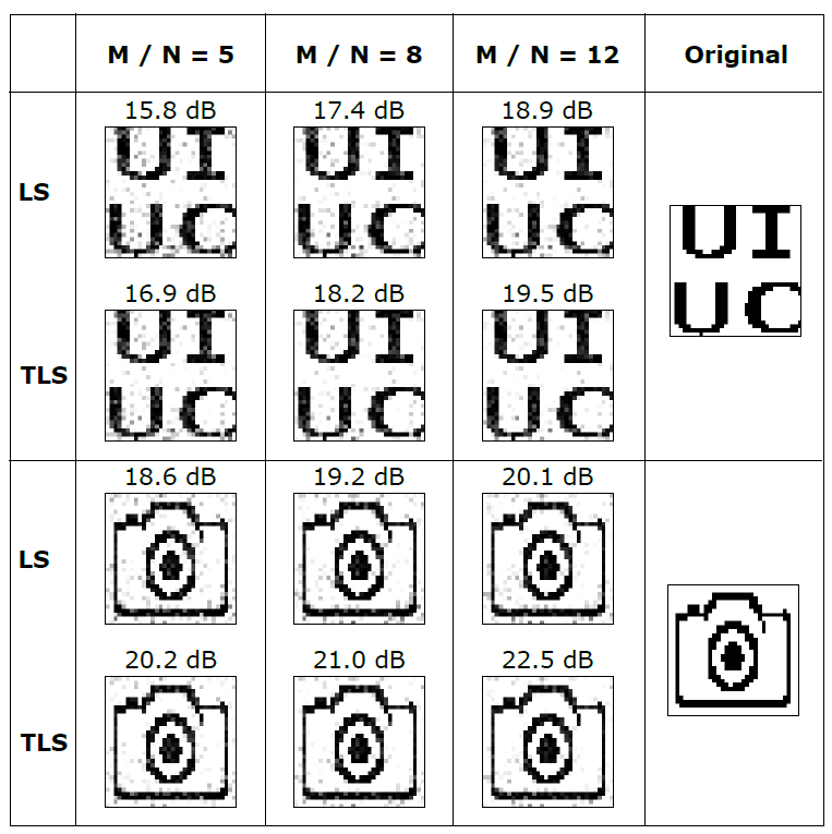
Many recent methods use a Least Squares (LS) approach with gradient decent. Such an approach only accounts for errors in the measurements, \( \abs{\vy}^2 \) . However, as our transmission matrix, \( \mA \), was calibrated from errorneous optical measurements, it also contains errors. With this in mind we have developed a Total Least Squares (TLS) approach which accounts for errors in both the measurements and transmission matrix.
The following figure shows that using our TLS approach results in better reconstructions than when a LS approach is used. The versampling ratio, \(\frac{M}{N}\), is varied and the reconstruction SNRs are reported:
Publications
2021
@article{gupta2021total,
  title={Total least squares phase retrieval},
  author={Gupta, Sidharth and Dokmani{\'c}, Ivan},
  journal={IEEE Transactions on Signal Processing},
  volume={70},
  pages={536--549},
  year={2021},
  publisher={IEEE}
}
2020
@inproceedings{gupta2020fast,
  title={Fast optical system identification by numerical interferometry},
  author={Gupta, Sidharth and Gribonval, R{\'e}mi and Daudet, Laurent and Dokmani{\'c}, Ivan},
  booktitle={ICASSP 2020-2020 IEEE International Conference on Acoustics, Speech and Signal Processing (ICASSP)},
  pages={1474--1478},
  year={2020},
  organization={IEEE}
}@article{huang2020solving,
title={Solving complex quadratic systems with full-rank random matrices},
author={Huang, Shuai and Gupta, Sidharth and Dokmani{\'c}, Ivan},
journal={IEEE Transactions on Signal Processing},
volume={68},
pages={4782--4796},
year={2020},
publisher={IEEE}
}2019
@article{gupta2019don,
  title={Don't take it lightly: Phasing optical random projections with unknown operators},
  author={Gupta, Sidharth and Gribonval, Remi and Daudet, Laurent and Dokmani{\'c}, Ivan},
  projectpage = {http://sada.dmi.unibas.ch/en/research/pr-optical-computing},
  journal={(NeurIPS) Advances in Neural Information Processing Systems},
  volume={32},
  pages={14855--14865},
  year={2019}
}@inproceedings{huang2019solving,
title={Solving complex quadratic equations with full-rank random Gaussian matrices},
author={Huang, Shuai* and Gupta, Sidharth* and Dokmani{\'c}, Ivan},
booktitle={ICASSP 2019-2019 IEEE International Conference on Acoustics, Speech and Signal Processing (ICASSP)},
pages={5596--5600},
year={2019},
organization={IEEE}
}2018
@article{huang2018reconstructing,
  title={Reconstructing point sets from distance distributions},
  author={Huang, Shuai and Dokmani{\'c}, Ivan},
  journal={arXiv preprint arXiv:1804.02465},
  year={2018}
}